Methods

Section Contents

1. Background
2. Learned dynamics model
3. Physics-based message-passing
4. Dataset
5. Training
6. Model assesment

Background

The following link to pages detailing background knowledge for those less farmilar with the computational and machine learning methods used here.

• Graph Neural Networks
• Symbolic Matrices

Learnt dynamics model

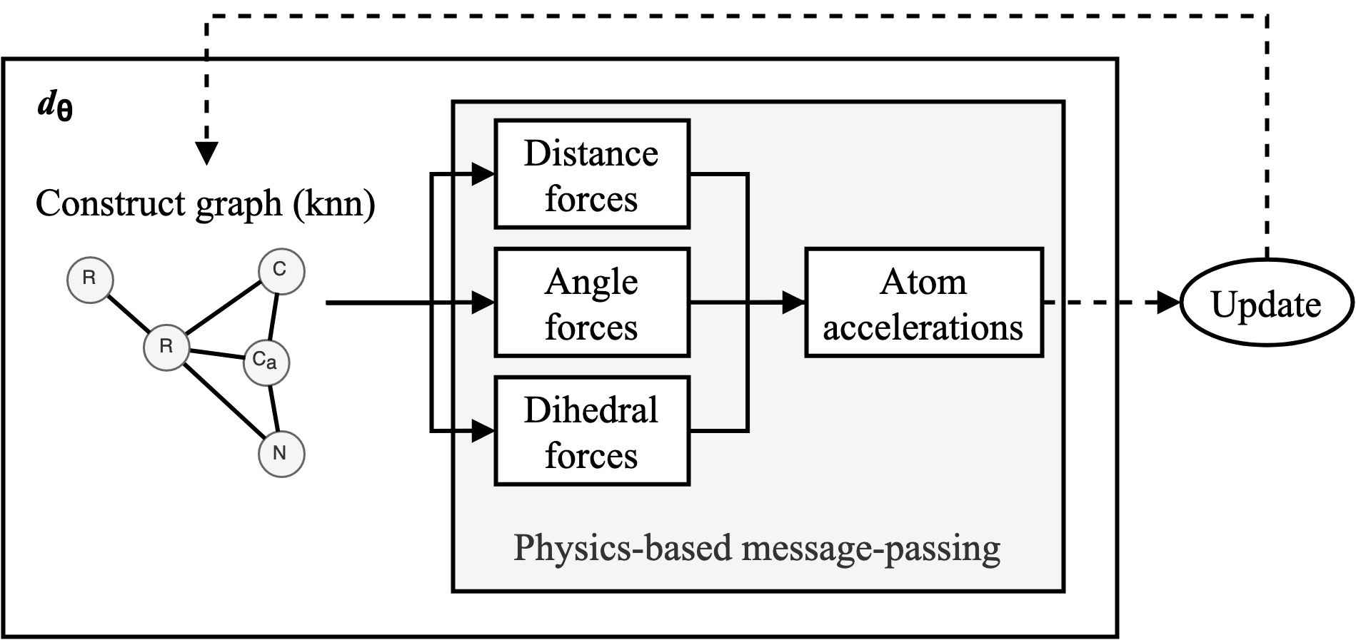
We construct a DMS simulator for proteins (as seen in Figure 1) where d_θ is outlined in Figure 2. For every N number of steps, the atoms enter d_θ as a set of points in space. Edges are drawn between the atoms using a fast KNN algorithm implemented in KeOps such that distance matrices only need to be computed symbolically. Our physics-based message-passing procedure (see next section) employs 3 separate sub-networks to predict the potentials of atom-atom interactions based on distances, angles and dihedrals respectively. Forces are calculated by taking the gradient of the potentials at the given distance/angle. Finally, all forces acting on every atom are summed and final atom accelerations are computed.

We use the same Verlet integrator as seen in Greener & Jones (2021) Greener, J. G. & Jones, D. T. (2021),
‘Differentiable molecular simulation can learn all the parameters in a coarse-grained force field for proteins’,
bioRxiv
doi:10.1101/2021.02.05.429941 as the Update function to compute the new velocities and coordinates. As the atoms are initialised with random starting velocities in every batch of training, the networks are forced to learn a dynamics model that can maintain the structure overtime (Figure 3). The simulator and the message-passing layers are implemented in Pytorch (Paszke et al. 2017Paszke, A., Gross, S., Chintala, S., Chanan, G., Yang, E., DeVito, Z., Lin, Z., Desmaison, A., Antiga, L. and Lerer, A., 2017. Automatic differentiation in pytorch.), making the whole function end-to-end differentiable.

Physics-based message-passing

We propose the use of a new GNN architecture, called physics-based message-passing (PBMP), which leverages our knowledge of the mechanics underlying molecular dynamics (Monasse & Boussinot 2014Monasse, B. & Boussinot, F. (2014), ‘Determination of forces from a potential in molecular dynamics’, arXiv preprint arXiv:1401.1181.) and the inductive biases of GNNs (Battaglia et al. 2018Battaglia, P. W., Hamrick, J. B., Bapst, V., Sanchez-Gonzalez, A., Zambaldi, V., Malinowski, M., Tacchetti, A., Raposo, D., Santoro, A., Faulkner, R. et al. (2018), ‘Relational inductive biases, deep learning, and graph networks’, arXiv preprint arXiv:1806.01261 ., Monti et al. 2017Monti, F., Boscaini, D., Masci, J., Rodola, E., Svoboda, J. & Bronstein, M. M. (2017), Geometric deep learning on graphs and manifolds using mixture model cnns, in ‘Proceedings of the IEEE conference on computer vision and pattern recognition’, pp. 5115–5124.). These physics-based equations could certainly be learnt by a neural network, but by integrating them into our message-passing procedure, we force the network to learn around these equations which makes our model interpretable. We define a basic PBMP as the following 4 equations:

\begin{equation} m_{ij} = \phi_e(h_i,h_j,e_{ij}) \end{equation} \begin{equation*} \overrightarrow{F_{ij}} = \psi_p(m_{ij}) \end{equation*} \begin{equation} \overrightarrow{F_i} = \sum_{j\in\mathcal{N}(i)}^{}\overrightarrow{F_{ij}} \end{equation} \begin{equation} \overrightarrow{a_i} = \overrightarrow{F_i}/mass_i \end{equation}

where h is the one-hot embeddings of the atom types, e_ij are the edge properties (e.g. Euclidean distance or bond angle), φ_e is a deep Multi Layer Perceptron (MLP) that constructs the one-dimensional messages mij, ψp is an equation derived from our knowledge of the physics of the systems. ψ_p in turn calculates the individual force vector (F_ij) that atom j exerts on atom i. F_i is the total force experienced by atom i and is the sum of all the forces exerted on it by the atoms in its neighbourhood Ɲ(i). The final accelerations experienced by the atoms, a_i, are calculated using Newton’s 2nd Law of Motion. The masses of the individual atoms, mass_i, are the only physical or chemical properties given to the model. Whilst the masses of the atoms could definitely be learnt in an end-to-end fashion, adding Eq 4 gives us interpretability when forces act on atoms of different masses. While PBMP shares multiple properties with conventional message-passing on graphs, our method does not apply an MLP over the node attributes (as this is the experienced force) and we add physics-based equations. We also only employ one layer of PBMP per time step.

In the distance submodule, e_ij also includes the absolute sequence seperation of the 2 atoms underconsideration. This allows for the model to learn differences between covalent bonds as well as local and global preferences. Eqs 1-4 describe the architecture of the distance sub-module shown in Figure 3. In the bond and dihedral angles sub-modules, we modify Equation 1 to take in 3 or 4 atom embeddings respectively. Thus, the ’messages’ constructed between multiple nodes/atoms encode the potential of that angle system. ψ_p in the angle and dihedral sub-modules can calculate the forces experienced by each atom correspondingly.

Full derivation of the equations used in ψ_p are provided in Monasse & Boussinot (2014)Monasse, B. & Boussinot, F. (2014), ‘Determination of forces from a potential in molecular dynamics’, arXiv preprint arXiv:1401.1181 .. However, in brief, the messages can be thought of as the scalar value describing the magnitude of the force between multiple atoms (be they bonded or in an angle/dihedral) and ψp recovers this into a 3D force vector to be applied to each atom. For example, in the case of distance forces, this is simply achieved by multiplying m_ij by the normalised vector difference between atoms i and j (norm(ij)).

Dataset

In this work we use the same dataset from Greener & Jones (2021) Greener, J. G. & Jones, D. T. (2021),
‘Differentiable molecular simulation can learn all the parameters in a coarse-grained force field for proteins’,
bioRxiv
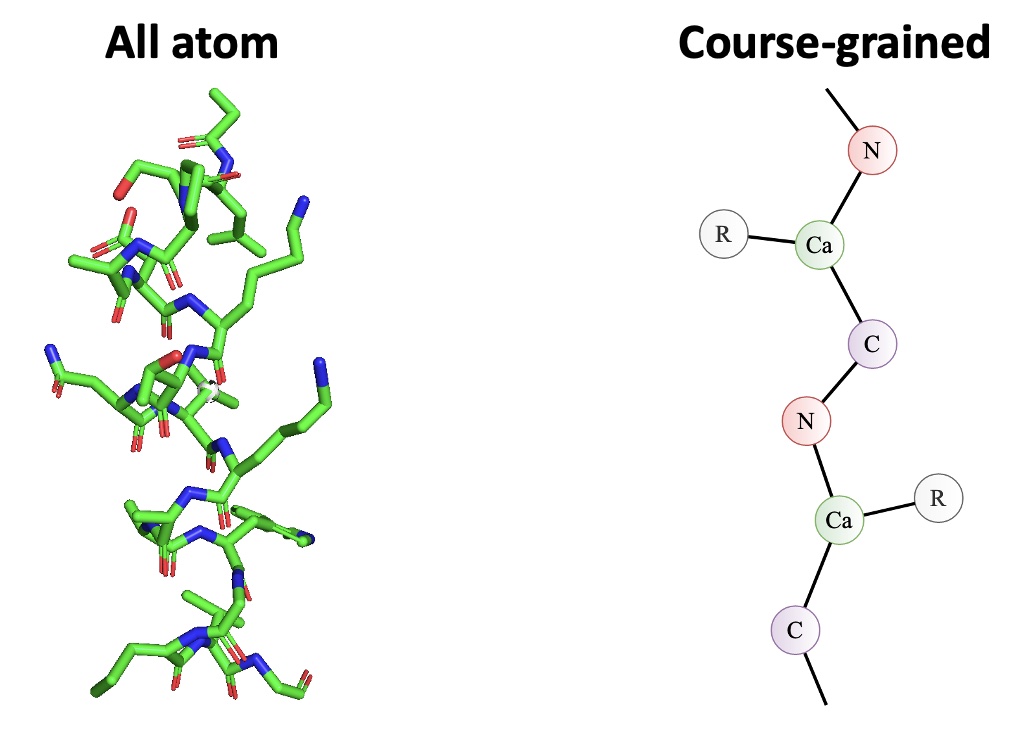
doi:10.1101/2021.02.05.429941 for training and evaluation. This dataset contains 2204 small protein structures (2004/200 train/test split) with a course-grained presentation (each residue has 4 atoms, Cα, C, N and side chain centroid) as seen in Figure 4. We use this datasets for fair comparisons, the quality of the structures (better than 2.5 Å resolutions and no missing internal residues) and small chain lengths (ideal for memory restrictions).

Training

All training was done on a NVIDIA Tesla V100 and took 32 GB of GPU memory for one forward pass using a batch size of 1. A starting temperature of 0.05, time step of 0.05, k of 20 and learning rate of 0.0005 were used over 1 epoch where each sample was simulated for 180 time steps during training. No thermostat was used during training.

Model assessment

Once we have trained the models, we can interpret the learnt dynamics by presenting the sub-networks with synthetic examples (e.g. 2 atoms at varying distances apart). These can then be used to graph potentials and compared to other force-fields (e.g. that in Greener & Jones (2021) Greener, J. G. & Jones, D. T. (2021),
‘Differentiable molecular simulation can learn all the parameters in a coarse-grained force field for proteins’,
bioRxiv
doi:10.1101/2021.02.05.429941 trained on the same data) and known statistics from chemical knowledge and the PDB (e.g. Mean Potential Force (Zhou & Zhou 2002Zhou, H. & Zhou, Y. (2002), ‘Distance-scaled, finite ideal-gas reference state improves structure-derived potentials of mean force for structure selection and stability prediction’, Protein science 11(11), 2714– 2726, doi.org/10.1110/ps.0217002.). This is only possible because we have integrated our knowledge of molecular dynamics into our neural network architecture.

After training, sample trajectories were generated over 10,000 steps (structure saved every 100 steps) with a time step of 0.02 and temperature of 0.02. We use lower temperature factors during testing as this is less likely to cause instability (i.e. an atom to move out of it's energy well). Folding of small proteins over 10,000s of steps was also attempted. Animations were made in PyMol (DeLano et al. 2002DeLano, W. L. et al. (2002), ‘Pymol: An open-source molecular graphics tool’, CCP4 Newsletter on protein crystallography 40(1), 82–92.) and plots were produced using Matplotlib (Hunter 2007Hunter, J. D. (2007), ‘Matplotlib: A 2d graphics environment’, IEEE Annals of the History of Computing 9(03), 90–95, doi.ieeecomputersociety.org/10.1109/MCSE.2007.55<).